Lesson 9 - Shortest Path
Shortest path represents the lowest path from a source vertex to a destination vertex on a weighted graph. The shortest path is a path that cumulatively has the lowest weight when combining the edges in the path.
Weighted Graph

A weighted graph is interesting because it has little to do with whether the graph is directed, undirected, or contains cycles. At its core, a weighted graph is a graph whose edges have some sort of value that is associated with them. The value that is attached to an edge is what gives the edge its “weight”.
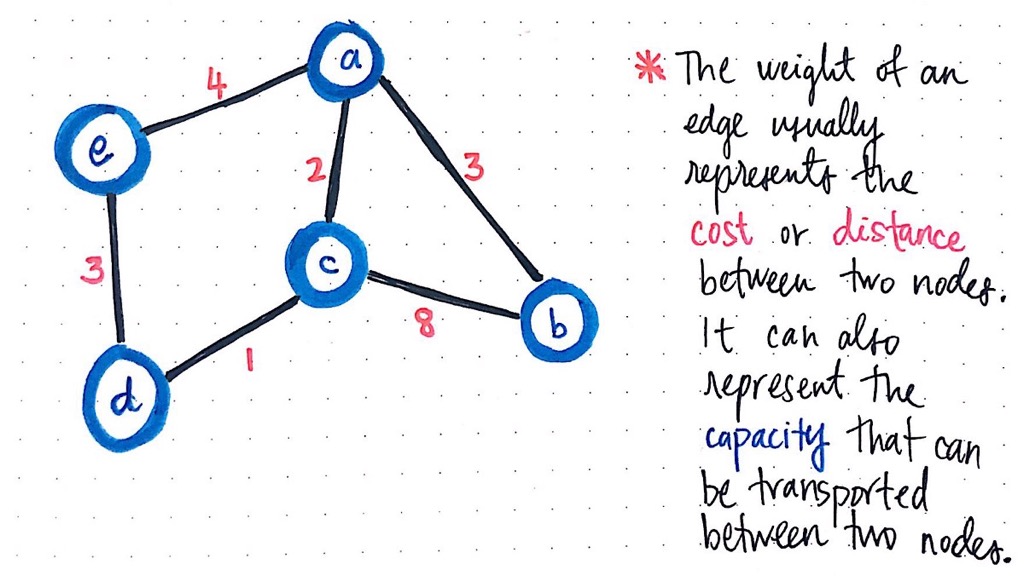
A common way to refer to the “weight” of a single edge is by thinking of it as the cost or distance between two nodes. In other words, to go from node a to node b has some sort of cost to it.
Or, if we think of the nodes like locations on a map, then the weight could instead be the distance between nodes a and b. Continuing with the map metaphor, the “weight” of an edge can also represent the capacity of what can be transported, or what can be moved between two nodes, a and b.
For example, in the example above, we could ascertain that the cost, distance, or capacity between the nodes c and b is weighted at 8.
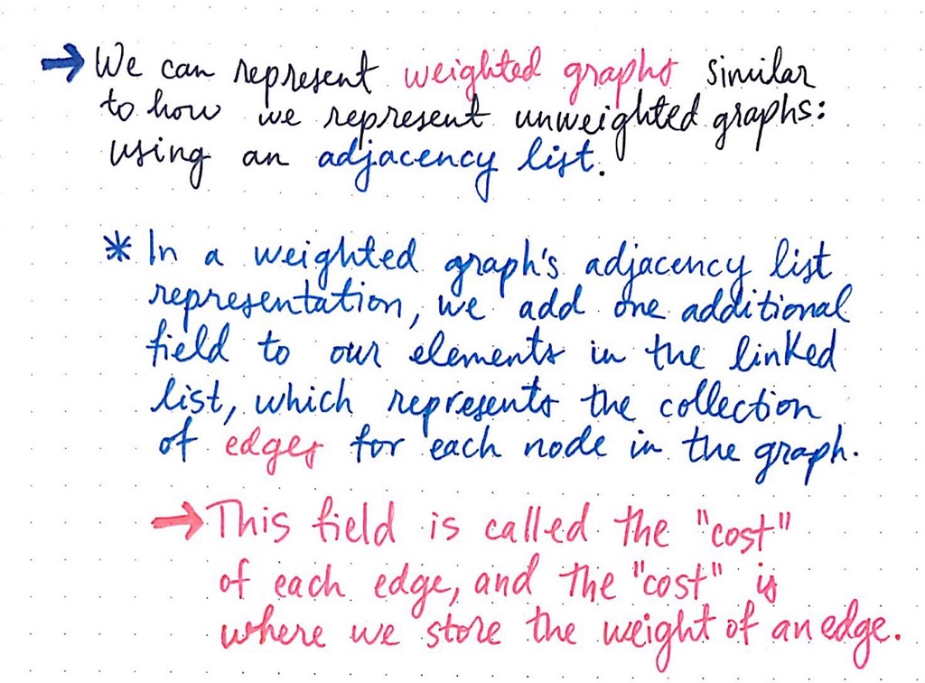
The weighted-ness of the edges is the only thing that sets weighted graphs apart from the unweighted graphs.
In fact, we probably already can imagine how we could represent one of these weighted graphs! A weighted graph can be represented with an adjacency list, with one added property: a field to store the cost/weight/distance of every edge in the graph.
For every single edge in our graph, we add the definition of the linked list that holds the edges so that every element in the linked list can contain two values, rather than just one. These two values will be the opposite node’s index, which is how we know where this edge connects to, as well as the weight that is associated with the edge.
Here’s what that same example weighted graph would look like in adjacency list format.
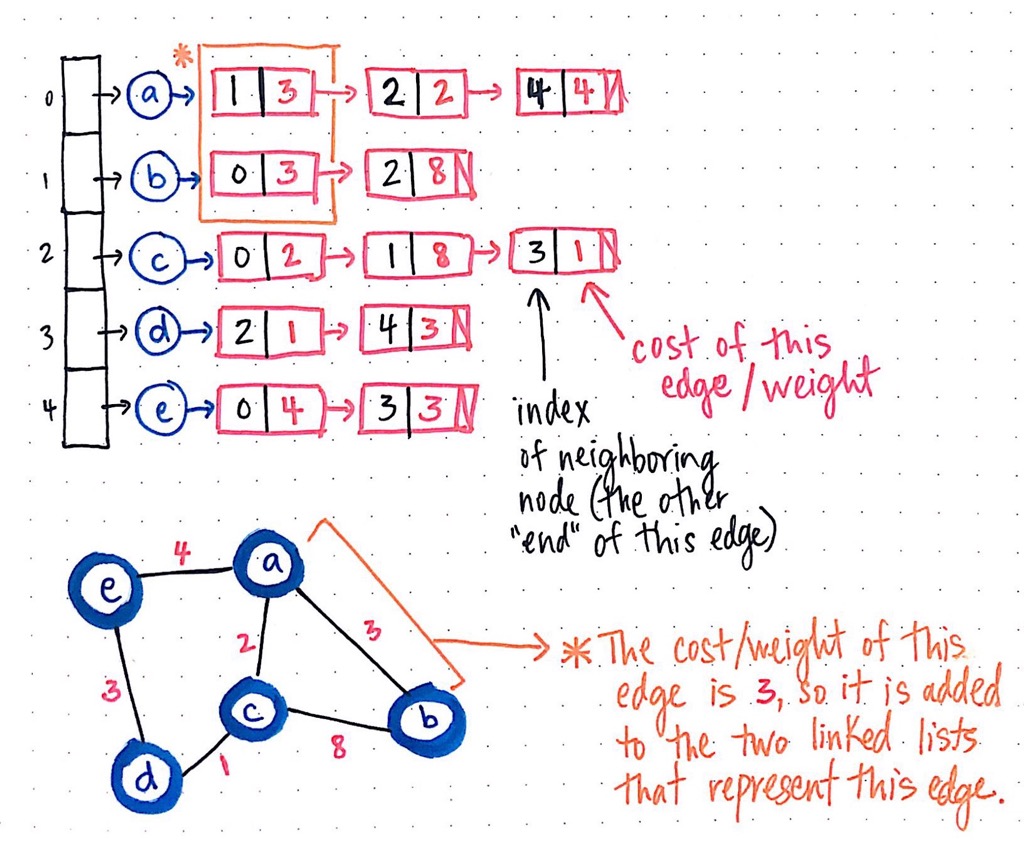
We notice two things about this graph representation: first, since it is an undirected graph, the edge between nodes a and b will appear twice — once in the edge list for node a and once in the edge list for node b. Second, in both instances that this edge is represented in either node’s respective edge list, there is a cost/weight that is stored in the linked list element that contains the reference to the adjacent node (in this case, either a or b).
Let us take a look at an example, and this will start to become more clear. In the simple directed, weighted graph below, we have a graph with three nodes (a, b, and c), with three directed, weighted edges.
Let us take a look at an example, and this will start to become more clear. In the simple directed, weighted graph below, we have a graph with three nodes (a, b, and c), with three directed, weighted edges.
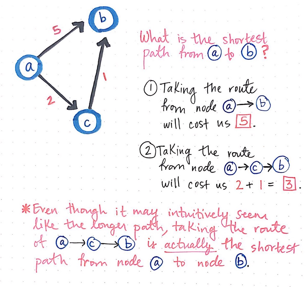
Looking at this graph, we might be able to quickly determine — without much hesitation — the quickest way to get from node ato node b. There is an edge between a and b, so that must be the quickest way, right?
Well, not exactly. Taking the weights of these edges into account, let’s take a deeper, second look. If we take the route from node a to node b, it will “cost us” 5. However, if we take the route from node a to node c to node b, then it will cost us only 3.
But why 3? Well, even though it may intuitively seem like a longer path, if we sum up the edges of going from node a to c and then from node c to b, we’ll see that the total cost ends up as 2 + 1, which is 3. It might mean that we’re traveling through two edges, but a cost of 3 is certainly preferable to a cost of 5!
In our three-node example graph, we could fairly easily look at the two possible routes between our origin and destination nodes. However, what if our graph was much bigger — let’s say twenty nodes? It wouldn’t have been nearly as easy for us to find the shortest path, taking into account the weights of our weighted graph. And what if we were talking about an even bigger graph? In fact, most graphs that we deal with are far bigger than twenty nodes. How feasible and scalable and efficient would it be for us to use a brute-force approach to solving this problem?
Dijkstra's Algorithm
Dijkstra’s algorithm was one of the first and most commonly studied algorithms for finding the shortest path. This algorithm is not just used to find the shortest path between two specific nodes in a graph data structure. Dijkstra’s algorithm can be used to determine the shortest path from one node in a graph to every other node within the same graph data structure, provided that the nodes are reachable from the starting node.
The algorithm is named after Edsger W. Dijkstra who first conceived the algorithm in 1956. Dijkstra's original algorithm does not use a min-priority queue and runs in O(V2)(where V is the number of nodes). The implementation based on a min-priority queue implemented by a Fibonacci heap and running in
In some fields, artificial intelligence in particular, Dijkstra's algorithm or a variant of it is known as uniform cost search and formulated as an instance of the more general idea of best-first search.
The algorithm is named after Edsger W. Dijkstra who first conceived the algorithm in 1956. Dijkstra's original algorithm does not use a min-priority queue and runs in O(V2)(where V is the number of nodes). The implementation based on a min-priority queue implemented by a Fibonacci heap and running in
O(E + Vlog(V)) (where E is the number of edges) is due to Fredman & Tarjan 1984. This is asymptotically the fastest known single-source shortest-path algorithm for arbitrary directed graphs with unbounded non-negative weights.In some fields, artificial intelligence in particular, Dijkstra's algorithm or a variant of it is known as uniform cost search and formulated as an instance of the more general idea of best-first search.
This algorithm will continue to run until all of the reachable vertices in a graph have been visited, which means that we could run Dijkstra’s algorithm, find the shortest path between any two reachable nodes, and then save the results somewhere. Once we run Dijkstra’s algorithm just once, we can look up our results from our algorithm again and again — without having to actually run the algorithm itself! The only time we’d ever need to re-run Dijkstra’s algorithm is if something about our graph data structure changed, in which case we’d end up re-running the algorithm to ensure that we still have the most up-to-date shortest paths for our particular data structure.
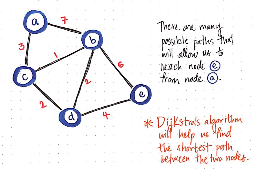
Consider the weighted, undirected graph above. Let us say that we want to find the shortest path from node a to node e. We know that we are going to start at node a, but we do not know if there is a path to reach it, or if there are many paths to reach it! In any case, we do not know which path will be the shortest one to get to node e, if such a path even exists.
Dijkstra’s algorithm does require a bit of initial setup. But, before we get to that, let us take a quick look at the steps and rules for running Dijkstra’s algorithm. In our example graph, we will start with node a as our starting node. However, the rules for running Dijkstra can be abstracted out so that they can be applied to every single node that we’ll traverse through and visit in an effort to find the shortest path.
Dijkstra’s algorithm does require a bit of initial setup. But, before we get to that, let us take a quick look at the steps and rules for running Dijkstra’s algorithm. In our example graph, we will start with node a as our starting node. However, the rules for running Dijkstra can be abstracted out so that they can be applied to every single node that we’ll traverse through and visit in an effort to find the shortest path.
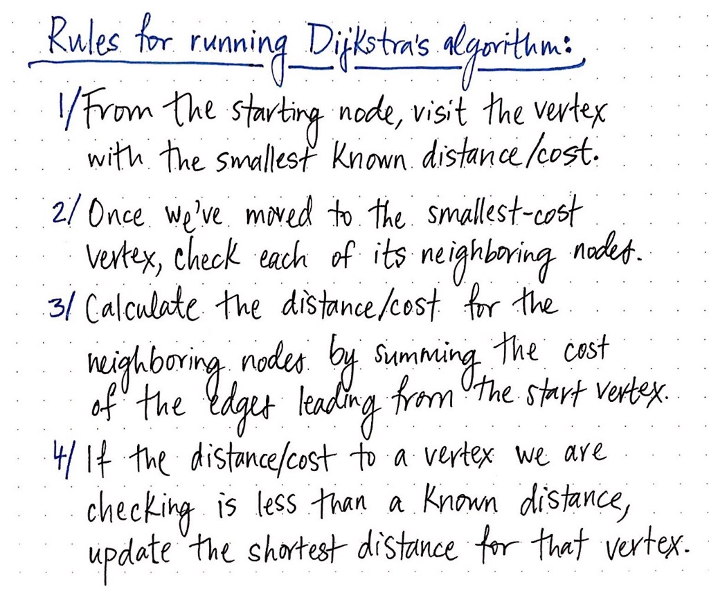
The abstracted rules are as follows:
- Every time that we set out to visit a new node, we will choose the node with the smallest known distance/cost to visit first.
- Once we have moved to the node we are going to visit, we will check each of its adjacent nodes.
- For each adjacent node, we will calculate the distance/cost for the adjacent nodes by summing the cost of the edges that lead to the node we are checking from the starting vertex.
- Finally, if the distance/cost to a node is less than a known distance, we update the shortest distance that we have on file for that vertex.
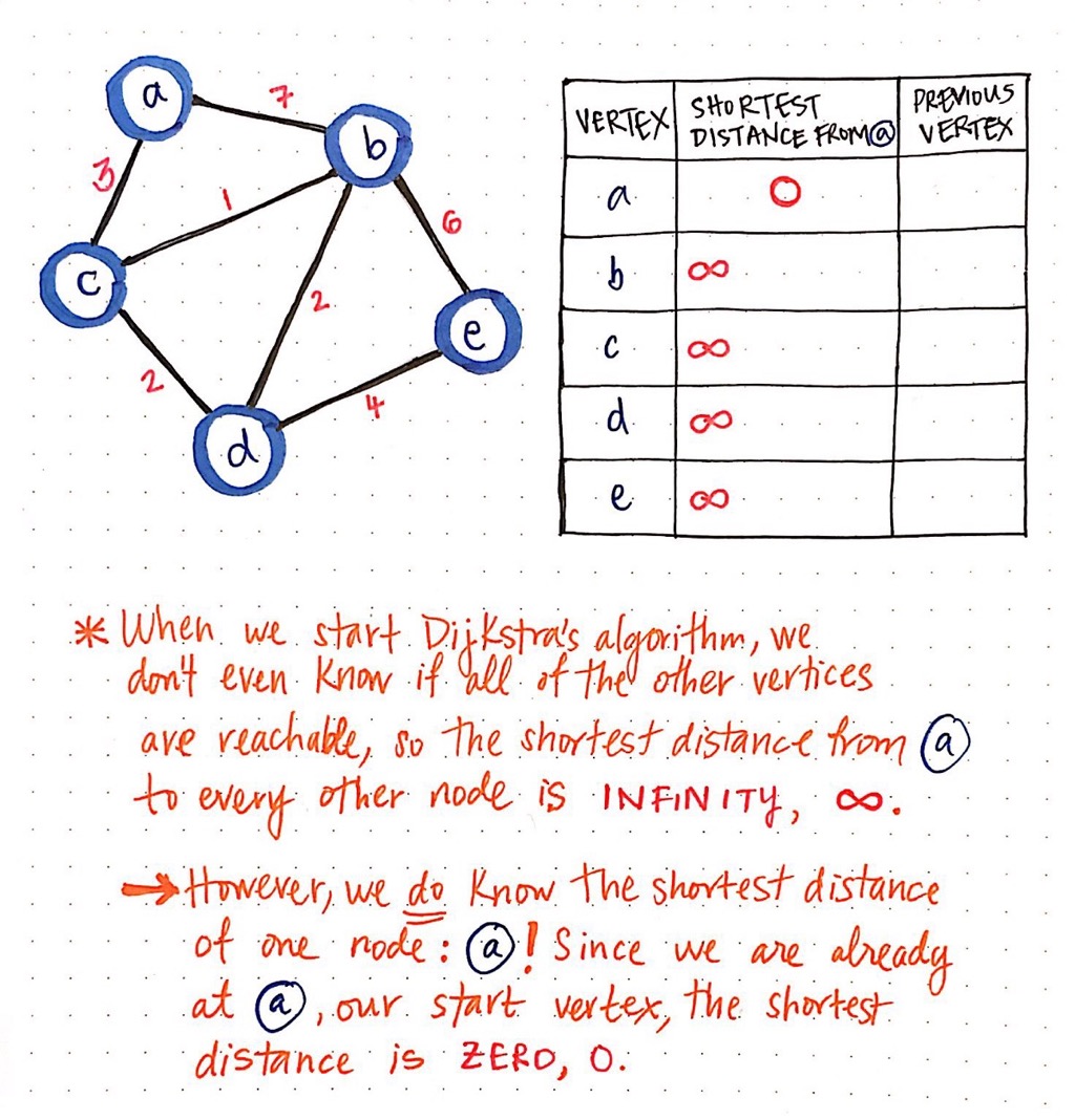
We will create a table to keep track of the shortest known distance to every vertex in our graph. We will also keep track of the previous vertex that we came from, before we “checked” the vertex that we are looking at currently.
Once we have our table all set up, we need to give it some values. When we start Dijkstra’s algorithm, we do not know anything at all! We do not even know if all of the other vertices that we have listed out (b, c, d, and e) are even reachable from our starting node a.
This means that, when we start out initially, the “shortest path from node a" is going to be infinity (∞). However, when we start out, we do know the shortest path for one node, and one node only: node a, our starting node! Since we start at node a, we are already there to begin with. So, the shortest distance from node a to node a is just 0!
Now that we have initialised our table, we need one other thing before we can run this algorithm: a way to keep track of which nodes we have or have not visited! We can do this pretty simply with two array structures: a visited array and an unvisited array.
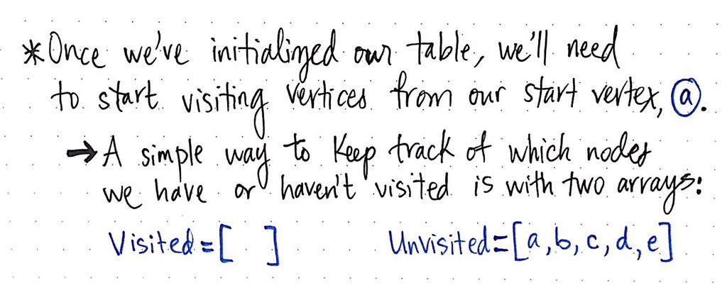
When we start out, we have not actually visited any nodes yet, so all of our nodes live inside of our unvisited array.
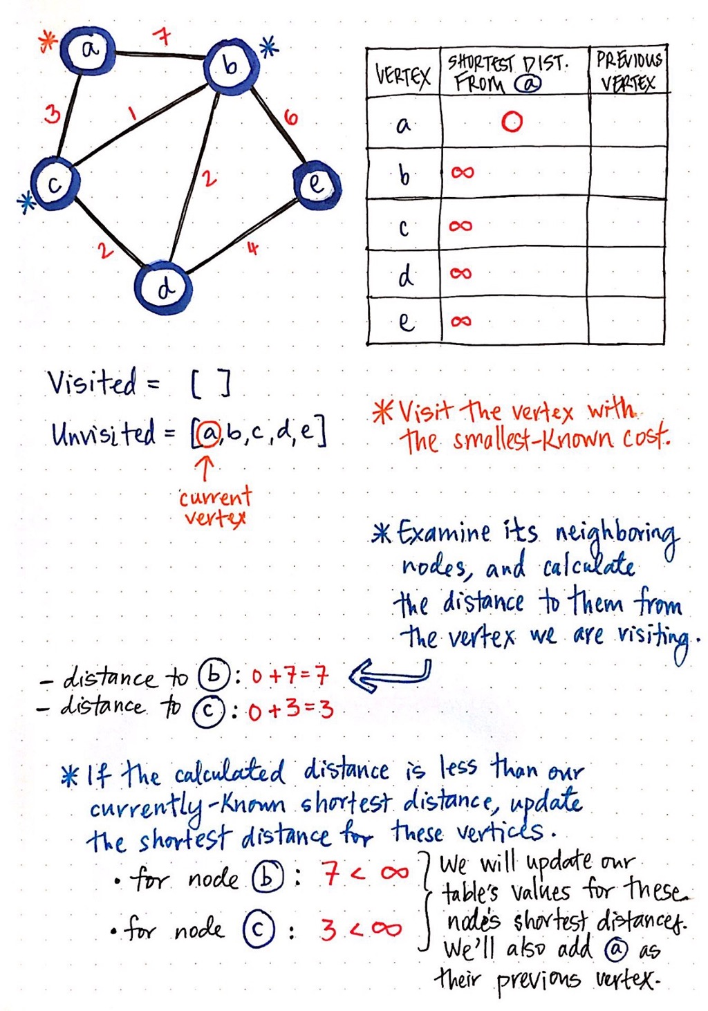
First, we visit the vertex with the smallest-known cost/distance. We can look at the column that tells us the shortest distance from a. Right now, every vertex has a distance of infinity (∞), except for a itself! So, we visit node a.
Next, we examine all adjacent nodes, and calculate the distance to them from the vertex that we are currently looking at (which is a). The distance to node b is the cost of a plus the cost to get to node b: in this case, 7. Similarly, the distance to node c is the cost of a plus the cost to get to node c: in this case, 3.
Finally, if the calculated distance is less than our currently-known shortest distance for these neighbouring nodes, we update our table's values with our new “shortest distance”. Currently, our table says that the shortest distance from a to b is ∞, and the same goes for the shortest distance from a to c. Since 7 is less than infinity, and 3 is less than infinity, we will update node b's shortest distance to 7, and node c's shortest distance to 3. We will also need to update the previous vertex of both b and c, since we need to keep a record of where we came from to get these paths! We update the previous vertex of b and c to a, since that is where we just came from.
Now, we are done checking the neighbours of node a, which means we can mark it as visited!
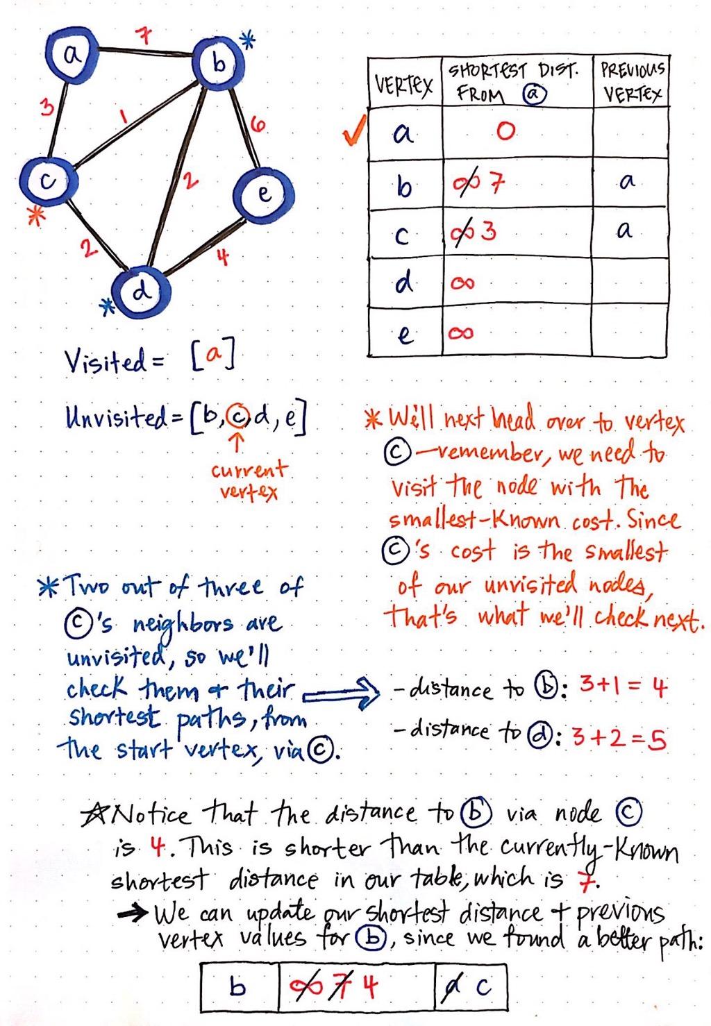
Again, we look at the node with the smallest cost that has not been visited yet. In this case, node c has a cost of 3, which is the smallest cost of all the unvisited nodes. So, node c becomes our current vertex.
We repeat the same procedure as before: check the unvisited adjacent vertices of node c, and calculate their shortest paths from our origin node, node a. The two neighbours of node c that have not been visited yet are node b and node d. The distance to node b is the cost of a plus the cost to get from node c to b: in this case, 4. The distance to node d is the cost of a plus the cost to get from node c to d: in this case, 5.
Now, compare these two “shortest distances” to the values that we have in our table. Right now, the distance to d is infinity, so we have certainly found a shorter-cost path here, with a value of 5. But what about the distance to node b? The distance to node b is currently marked as 7 in our table. But, we have found a shorter path to b, which goes through c, and has a cost of only 4. So, we update our table with our shorter paths!
We also need to add vertex c as the previous vertex of node d. Notice that node b already has a previous vertex, since we found a path before, which we now know is not actually the shortest. We just cross out the previous vertex for node b, and replace it with the vertex which, as we now know, has the shorter path: node c.
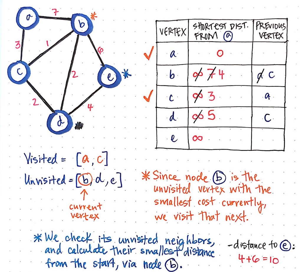
So far we have visited both node a and c. So, which node do we visit next?
Again, we visit the node that has the smallest cost; in this case, that looks to be node b, with a cost of 4.
We check its unvisited neighbour (it only has one, node e), and calculate the distance to e, from the origin node, via our current vertex, b.
If we sum the cost of b, which is 4, with the cost that it takes to get from b to e, we see that this costs us 6. Thus, we end up with a total cost of 10 as the shortest-known distance to e, from the starting vertex, via our current node.
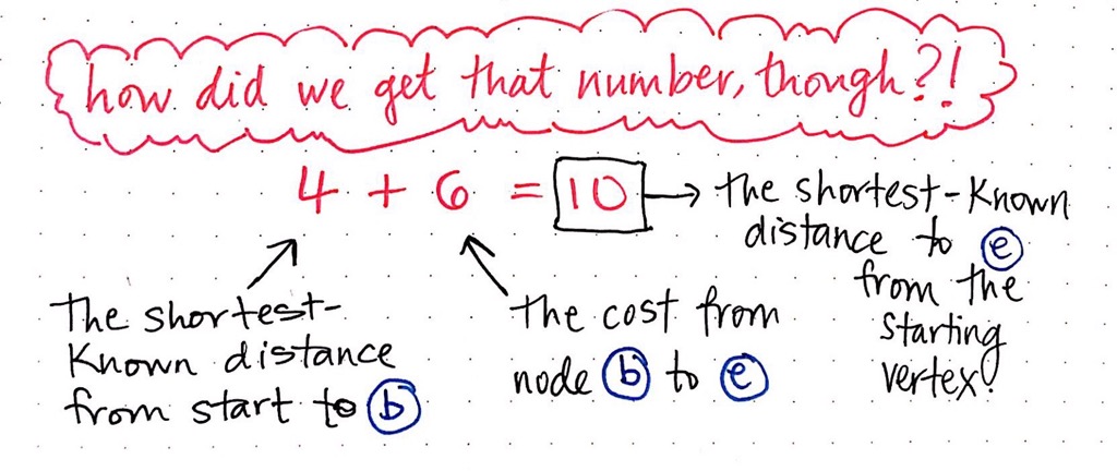
How did we get that number? We can break it down into parts. Remember, no matter which vertex we are looking at, we always want to sum the shortest-known distance from our start to our current vertex. In simpler terms, we are going to look at the “shortest distance” value in our table, which will give us, in this example, the value 4. Then, we look at the cost from our current vertex to the neighbour that we are examining. In this case, the cost from b to e is 6, so we add that to 4.
Thus,
Thus,
6 + 4 = 10 is our shortest-known distance to node e from our starting vertex a.A* Algorithm
The A* algorithm is often used in video games to enable characters to navigate the world.
Some problems can be solved by representing the world in the initial state, and then for each action we can perform on the world we generate states for what the world would be like if we did so. If you do this until the world is in the state that we specified as a solution, then the route from the start to this goal state is the solution to your problem.
A node is a state that the problem's world can be in. In pathfinding a node would be just a 2d coordinate of where we are at the present time.
Next all the nodes are arranged in a graph where links between nodes represent valid steps in solving the problem. These links are known as edges.
State space search, then, is solving a problem by beginning with the start state, and then for each node we expand all the nodes beneath it in the graph by applying all the possible moves that can be made at each point.
At this point we introduce an important concept, the heuristic. This is like an algorithm, but with a key difference. An algorithm is a set of steps which you can follow to solve a problem, which always works for valid input. For example you could probably write an algorithm yourself for multiplying two numbers together on paper. A heuristic is not guaranteed to work but is useful in that it may solve a problem for which there is no algorithm.
We need a heuristic to help us cut down on this huge search problem. What we need is to use our heuristic at each node to make an estimate of how far we are from the goal. In pathfinding we know exactly how far we are, because we know how far we can move each step, and we can calculate the exact distance to the goal.
When looking at each node in the graph, we now have an idea of a heuristic, which can estimate how close the state is to the goal. Another important consideration is the cost of getting to where we are. In the case of pathfinding we often assign a movement cost to each edge. If we wanted to differentiate between terrain types we may give higher costs to grass and mud than to newly made road. When looking at a node we want to add up the cost of what it took to get here, and this is simply the sum of the cost of this node and all those that are above it in the graph.
In a video game, or some other pathfinding scenario, you want to search a state space and find out how to get from somewhere you are to somewhere you want to be, without bumping into walls or going too far. The A* algorithm will not only find a path, if there is one, but it will find the shortest path. A state in pathfinding is simply a position in the world. In the example of a maze game like Pacman you can represent where everything is using a simple 2d grid. The start state for a ghost say, would be the 2d coordinate of where the ghost is at the start of the search. The goal state would be where pacman is so we can go and eat him.
At each stage, the A* algorithm uses the following function to determine the next edge to try:
The heuristic can be used to control A*’s behaviour.
Technically, the A* algorithm should be called simply A if the heuristic is an underestimate of the actual cost. However, we will continue to call it A* because the implementation is the same and the game programming community does not distinguish A from A*.
So we have an interesting situation in that we can decide what we want to get out of A*. At exactly the right point, we will get shortest paths really quickly. If we are too low, then we will continue to get shortest paths, but it will slow down. If we are too high, then we give up shortest paths, but A* will run faster.
In a game, this property of A* can be very useful. For example, you may find that in some situations, you would rather have a “good” path than a “perfect” path. To shift the balance between
A*’s ability to vary its behaviour based on the heuristic and cost functions can be very useful in a game. The tradeoff between speed and accuracy can be exploited to make your game faster. For most games, you don’t really need the best path between two points. You need something that is close. What you need may depend on what’s going on in the game, or how fast the computer is.
Suppose your game has two types of terrain, Flat and Mountain, and the movement costs are 1 for flat land and 3 for mountains, A* is going to search three times as far along flat land as it does along mountainous land. This is because it is possible that there is a path along flat terrain that goes around the mountains. You can speed up A*’s search by using 1.5 as the heuristic distance between two map spaces. A* will then compare 3 to 1.5, and it won’t look as bad as comparing 3 to 1. It is not as dissatisfied with mountainous terrain, so it will not spend as much time trying to find a way around it. Alternatively, you can speed up up A*’s search by decreasing the amount it searches for paths around mountains―tell A* that the movement cost on mountains is 2 instead of 3. Now it will search only twice as far along the flat terrain as along mountainous terrain. Either approach gives up ideal paths to get something quicker.
The choice between speed and accuracy does not have to be static. You can choose dynamically based on the CPU speed, the fraction of time going into pathfinding, the number of units on the map, the importance of the unit, the size of the group, the difficulty level, or any other factor. One way to make the tradeoff dynamic is to build a heuristic function that assumes the minimum cost to travel one grid space is 1 and then build a cost function that scales:
If alpha is 0, then the modified cost function will always be 1. At this setting, terrain costs are completely ignored, and A* works at the level of simple passable/unpassable grid spaces. If alpha is 1, then the original cost function will be used, and you get the full benefit of A*. You can set alpha anywhere in between.
You should also consider switching from the heuristic returning the absolute minimum cost to returning the expected minimum cost. For example, if most of your map is grasslands with a movement cost of 2 but some spaces on the map are roads with a movement cost of 1, then you might consider having the heuristic assume no roads, and return
The choice between speed and accuracy does not have to be global. You can choose some things dynamically based on the importance of having accuracy in some region of the map. For example, it may be more important to choose a good path near the current location, on the assumption that we might end up recalculating the path or changing direction at some point, so why bother being accurate about the faraway part of the path? Or perhaps it’s not so important to have the shortest path in a safe area of the map, but when sneaking past an enemy village, safety and quickness are essential.
A* computes
On a grid, there are well-known heuristic functions to use.
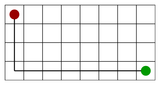
Use the distance heuristic that matches the allowed movement:
Multiply the distance in steps by the minimum cost for a step. For example, if you are measuring in metres, the distance is 3 squares, and each square is 15 metres, then the heuristic would return 3 ⨉ 15 = 45 metres. If you are measuring in time, the distance is 3 squares, and each square takes at least 4 minutes to cross, then the heuristic would return 3 ⨉ 4 = 12 minutes. The units (metres, minutes, etc.) returned by the heuristic should match the units used by the cost function.
The sum of absolute values of differences in the goal’s x and y coordinates and the current cell’s x and y coordinates respectively
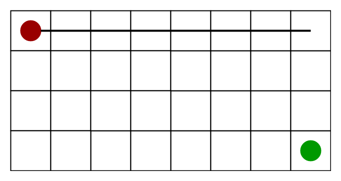
The maximum of absolute values of differences in the goal’s x and y coordinates and the current cell’s x and y coordinates respectively, i.e.
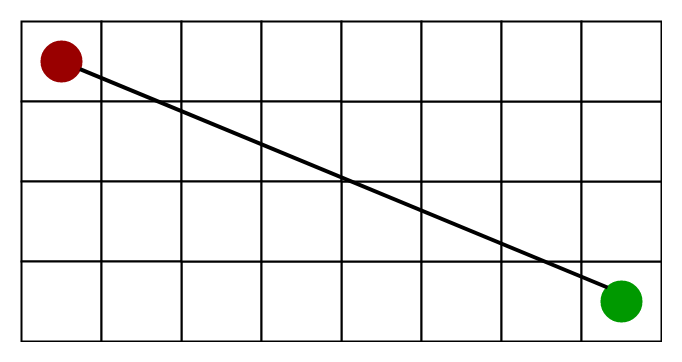
The distance between the current cell and the goal cell using the distance formula
h = sqrt( (current_cell.x – goal.x)2 + (current_cell.y – goal.y)2 )
A heuristic that has the exact distance is ideal for making A* fast but it is usually impractical. We can often preprocess the graph to construct an approximate distance, and use that approximation in the A* heuristic.
ALT A* uses “landmarks” and triangle inequality to preprocess the pathfinding graph in order to make pathfinding much faster. It is surprisingly simple to implement, sometimes under 15 lines of code, and produces impressive speedups.
The name “landmark” is a little misleading. These points need to be placed on the outer edges of the map. Some authors call it “differential heuristics”.
The landmark approach stores lots of data that could be compressed. You can store a lot more landmarks in the same space, so you get improved heuristic values.
The A* algorithm is fairly simple. There are two sets, OPEN and CLOSED. The OPEN set contains those nodes that are candidates for examining. Initially, the OPEN set contains only one element: the starting position. The CLOSED set contains those nodes that have already been examined. Initially, the CLOSED set is empty. Graphically, the OPEN set is the “frontier” and the CLOSED set is the “interior” of the visited areas. Each node also keeps a pointer to its parent node so that we can determine how it was found.
There is a main loop that repeatedly pulls out the best node
See detail implementation notes on this site.
State space search
Some problems can be solved by representing the world in the initial state, and then for each action we can perform on the world we generate states for what the world would be like if we did so. If you do this until the world is in the state that we specified as a solution, then the route from the start to this goal state is the solution to your problem.
Terminology
A node is a state that the problem's world can be in. In pathfinding a node would be just a 2d coordinate of where we are at the present time.
Next all the nodes are arranged in a graph where links between nodes represent valid steps in solving the problem. These links are known as edges.
State space search, then, is solving a problem by beginning with the start state, and then for each node we expand all the nodes beneath it in the graph by applying all the possible moves that can be made at each point.
Heuristics and Algorithms
At this point we introduce an important concept, the heuristic. This is like an algorithm, but with a key difference. An algorithm is a set of steps which you can follow to solve a problem, which always works for valid input. For example you could probably write an algorithm yourself for multiplying two numbers together on paper. A heuristic is not guaranteed to work but is useful in that it may solve a problem for which there is no algorithm.
We need a heuristic to help us cut down on this huge search problem. What we need is to use our heuristic at each node to make an estimate of how far we are from the goal. In pathfinding we know exactly how far we are, because we know how far we can move each step, and we can calculate the exact distance to the goal.
Cost
When looking at each node in the graph, we now have an idea of a heuristic, which can estimate how close the state is to the goal. Another important consideration is the cost of getting to where we are. In the case of pathfinding we often assign a movement cost to each edge. If we wanted to differentiate between terrain types we may give higher costs to grass and mud than to newly made road. When looking at a node we want to add up the cost of what it took to get here, and this is simply the sum of the cost of this node and all those that are above it in the graph.
Pathfinding
In a video game, or some other pathfinding scenario, you want to search a state space and find out how to get from somewhere you are to somewhere you want to be, without bumping into walls or going too far. The A* algorithm will not only find a path, if there is one, but it will find the shortest path. A state in pathfinding is simply a position in the world. In the example of a maze game like Pacman you can represent where everything is using a simple 2d grid. The start state for a ghost say, would be the 2d coordinate of where the ghost is at the start of the search. The goal state would be where pacman is so we can go and eat him.
Heuristic
At each stage, the A* algorithm uses the following function to determine the next edge to try:
f(n) = g(n) + h(n)g(n)represents the exact cost of the path from the starting point to any vertexnh(n)represents the heuristic estimated cost from vertexnto the goal
The heuristic can be used to control A*’s behaviour.
- At one extreme, if
h(n)is 0, then onlyg(n)plays a role, and A* turns into Dijkstra’s Algorithm, which is guaranteed to find a shortest path. - If
h(n)is always lower than (or equal to) the cost of moving fromnto the goal, then A* is guaranteed to find a shortest path. The lowerh(n)is, the more node A* expands, making it slower. - If
h(n)is exactly equal to the cost of moving fromnto the goal, then A* will only follow the best path and never expand anything else, making it very fast. Although you can not make this happen in all cases, you can make it exact in some special cases. It is nice to know that given perfect information, A* will behave perfectly. - If
h(n)is sometimes greater than the cost of moving fromnto the goal, then A* is not guaranteed to find a shortest path, but it can run faster. - At the other extreme, if
h(n)is very high relative tog(n), then onlyh(n)plays a role, and A* turns into Greedy Best-First-Search.
Note:
Technically, the A* algorithm should be called simply A if the heuristic is an underestimate of the actual cost. However, we will continue to call it A* because the implementation is the same and the game programming community does not distinguish A from A*.
So we have an interesting situation in that we can decide what we want to get out of A*. At exactly the right point, we will get shortest paths really quickly. If we are too low, then we will continue to get shortest paths, but it will slow down. If we are too high, then we give up shortest paths, but A* will run faster.
In a game, this property of A* can be very useful. For example, you may find that in some situations, you would rather have a “good” path than a “perfect” path. To shift the balance between
g(n) and h(n), you can modify either one.Speed or accuracy?
A*’s ability to vary its behaviour based on the heuristic and cost functions can be very useful in a game. The tradeoff between speed and accuracy can be exploited to make your game faster. For most games, you don’t really need the best path between two points. You need something that is close. What you need may depend on what’s going on in the game, or how fast the computer is.
Suppose your game has two types of terrain, Flat and Mountain, and the movement costs are 1 for flat land and 3 for mountains, A* is going to search three times as far along flat land as it does along mountainous land. This is because it is possible that there is a path along flat terrain that goes around the mountains. You can speed up A*’s search by using 1.5 as the heuristic distance between two map spaces. A* will then compare 3 to 1.5, and it won’t look as bad as comparing 3 to 1. It is not as dissatisfied with mountainous terrain, so it will not spend as much time trying to find a way around it. Alternatively, you can speed up up A*’s search by decreasing the amount it searches for paths around mountains―tell A* that the movement cost on mountains is 2 instead of 3. Now it will search only twice as far along the flat terrain as along mountainous terrain. Either approach gives up ideal paths to get something quicker.
The choice between speed and accuracy does not have to be static. You can choose dynamically based on the CPU speed, the fraction of time going into pathfinding, the number of units on the map, the importance of the unit, the size of the group, the difficulty level, or any other factor. One way to make the tradeoff dynamic is to build a heuristic function that assumes the minimum cost to travel one grid space is 1 and then build a cost function that scales:
g'(n) = 1 + alpha * (g(n) - 1)If alpha is 0, then the modified cost function will always be 1. At this setting, terrain costs are completely ignored, and A* works at the level of simple passable/unpassable grid spaces. If alpha is 1, then the original cost function will be used, and you get the full benefit of A*. You can set alpha anywhere in between.
You should also consider switching from the heuristic returning the absolute minimum cost to returning the expected minimum cost. For example, if most of your map is grasslands with a movement cost of 2 but some spaces on the map are roads with a movement cost of 1, then you might consider having the heuristic assume no roads, and return
2 * distance.The choice between speed and accuracy does not have to be global. You can choose some things dynamically based on the importance of having accuracy in some region of the map. For example, it may be more important to choose a good path near the current location, on the assumption that we might end up recalculating the path or changing direction at some point, so why bother being accurate about the faraway part of the path? Or perhaps it’s not so important to have the shortest path in a safe area of the map, but when sneaking past an enemy village, safety and quickness are essential.
Scale
A* computes
f(n) = g(n) + h(n). To add two values, those two values need to be at the same scale. If g(n) is measured in hours and h(n) is measured in metres, then A* is going to consider g or h too much or too little, and you either will not get as good paths or you A* will run slower than it could.Heuristics for grid maps
On a grid, there are well-known heuristic functions to use.
Use the distance heuristic that matches the allowed movement:
- On a square grid that allows 4 directions of movement, use Manhattan distance.
- On a square grid that allows 8 directions of movement, use Diagonal distance.
- On a square grid that allows any direction of movement, you might or might not want Euclidean distance.
- On a hexagon grid that allows 6 directions of movement, use Manhattan distance adapted to hexagonal grids.
Multiply the distance in steps by the minimum cost for a step. For example, if you are measuring in metres, the distance is 3 squares, and each square is 15 metres, then the heuristic would return 3 ⨉ 15 = 45 metres. If you are measuring in time, the distance is 3 squares, and each square takes at least 4 minutes to cross, then the heuristic would return 3 ⨉ 4 = 12 minutes. The units (metres, minutes, etc.) returned by the heuristic should match the units used by the cost function.
Manhattan Distance
The sum of absolute values of differences in the goal’s x and y coordinates and the current cell’s x and y coordinates respectively
h = abs(current_cell.x – goal.x) + abs (current_cell.y – goal.y)
Diagonal Distance
The maximum of absolute values of differences in the goal’s x and y coordinates and the current cell’s x and y coordinates respectively, i.e.
h = max { abs(current_cell.x – goal.x),abs(current_cell.y – goal.y) }
Euclidean Distance
The distance between the current cell and the goal cell using the distance formula
h = sqrt( (current_cell.x – goal.x)2 + (current_cell.y – goal.y)2 )

Approximate heuristics
A heuristic that has the exact distance is ideal for making A* fast but it is usually impractical. We can often preprocess the graph to construct an approximate distance, and use that approximation in the A* heuristic.
ALT A* uses “landmarks” and triangle inequality to preprocess the pathfinding graph in order to make pathfinding much faster. It is surprisingly simple to implement, sometimes under 15 lines of code, and produces impressive speedups.
The name “landmark” is a little misleading. These points need to be placed on the outer edges of the map. Some authors call it “differential heuristics”.
The landmark approach stores lots of data that could be compressed. You can store a lot more landmarks in the same space, so you get improved heuristic values.
Implementation
The A* algorithm is fairly simple. There are two sets, OPEN and CLOSED. The OPEN set contains those nodes that are candidates for examining. Initially, the OPEN set contains only one element: the starting position. The CLOSED set contains those nodes that have already been examined. Initially, the CLOSED set is empty. Graphically, the OPEN set is the “frontier” and the CLOSED set is the “interior” of the visited areas. Each node also keeps a pointer to its parent node so that we can determine how it was found.
There is a main loop that repeatedly pulls out the best node
n from OPEN (the node with the lowest f value) and examines it. If n is the goal, then we are done. Otherwise, node n is removed from OPEN and added to CLOSED. Then, its neighbours n′ are examined. A neighbour that is in CLOSED has already been visited and is ignored. A neighbour that is in OPEN is enqueued to be visited. Otherwise, we add it to OPEN, with its parent set to n. The path cost to n′, g(n′), will be set to g(n) + movementcost(n, n′).See detail implementation notes on this site.
