Quicksort

Quicksort is a fast sorting algorithm, which is used not only for educational purposes, but also widely applied in practice. On the average, it has O(n log n) complexity, making quicksort suitable for sorting big data volumes.

Algorithm

A divide-and-conquer strategy is used in quicksort.

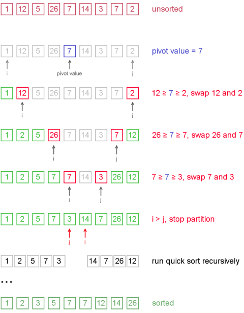
1. Choose a pivot value. We take the value of the middle element as pivot value, but it can be any value, which is in range of sorted values, even if it is not present in the data set. Note that in our implementation, we take the easy option of using the first value in the range specified as the pivot value. Assuming the input data set is unsorted, this is just as valid as a median pivot value, and makes the implementation a bit simpler.
2. Partition. Rearrange elements in such a way, that all elements which are lesser than the pivot go to the left part of the data set and all elements greater than the pivot, go to the right part of the data set. Values equal to the pivot can stay in any part of the data set. Notice, that the data set may be divided in non-equal parts.
3. Sort both parts. Apply quicksort algorithm recursively to the left and the right parts.

Partition algorithm in detail

There are two indices i and j and at the very beginning of the partition algorithm i points to the first element in the data set and j points to the last one. Then algorithm moves i forward, until an element with value greater or equal to the pivot is found. Index j is moved backward, until an element with value lesser or equal to the pivot is found. If i ≤ j then they are swapped and i steps to the next position (i + 1), j steps to the previous one (j - 1). Algorithm stops, when i becomes greater than j.

After partition, all values before i-th element are less or equal than the pivot and all values after j-th element are greater or equal to the pivot.

Example. Sort {1, 12, 5, 26, 7, 14, 3, 7, 2} using quicksort.

Notice, that we show here only the first recursion step, in order not to make example too long. But, in fact, {1, 2, 5, 7, 3} and {14, 7, 26, 12} are sorted then recursively.

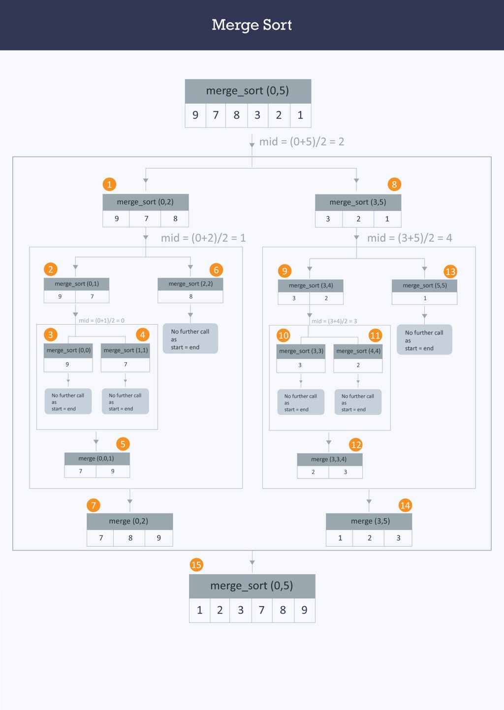
In computer science, merge sort (also commonly spelled mergesort) is an efficient, general-purpose, comparison-based sorting algorithm. Most implementations produce a stable sort, which means that the implementation preserves the input order of equal elements in the sorted output. Mergesort is a divide and conquer algorithm that was invented by John von Neumann in 1945. A detailed description and analysis of bottom-up mergesort appeared in a report by Goldstine and von Neumann as early as 1948.

Algorithm

Conceptually, a merge sort works as follows:

• Divide the unsorted data set into n data sets, each containing 1 element (a data set of 1 element is considered sorted).
• Repeatedly merge the sub sets to produce new sorted data sets until there is only 1 data set remaining. This will be the sorted data set.

The worst-case time complexity of the algorithm is Ο(n log n). Similar techniques are used to sort data stored in disk (external sort). Merge sort is also used as the last step in modern algorithms that need to sort large volumes of data (billions of items). When sorting large data sets, the first step is to partition the data and use some other algorithm to sort the smaller partitions, and then in the final phase use merge sort to produce the final sorted data set.

Illustration

To understand the merge sort algorithm, let us start with an unsorted data set such as −

Merge sort first divides the whole data set iteratively into equal halves until atomic/single values are encountered. In the first step an array of 8 items is divided into two arrays of size 4.

This does not change the sequence of appearance of items in the original. Now we divide these two arrays into halves.

We further divide these arrays and we achieve the target atomic values which can no longer be divided.

Now, we combine them in exactly the same manner as they were broken down. Please note the colour codes given to these lists.

We first compare the element for each list and then combine them into another list in a sorted manner. We see that 14 and 33 are in sorted positions. We compare 27 and 10 and in the target list of 2 values we put 10 first, followed by 27. We change the order of 19 and 35 whereas 42 and 44 are placed sequentially.

In the next iteration of the combining phase, we compare the data sets of two values each and merge them into two final data sets of four values each. As in the previous step, each of the two resulting data sets are sorted.

After the final merging, the we get the fully sorted data set as −