Lesson 17 - Tree

Trees are one of the most important nonlinear data structures in computing. Tree structures are indeed a breakthrough in data organisation, for they allow us to implement a host of algorithms much faster than when using linear data structures, such as lists, vectors, and sequences. Trees also provide a natural organisation for data, and consequently have become ubiquitous structures in file systems, graphical user interfaces, databases, Web sites, and other computer systems.

The relationships in a tree are hierarchical, with some objects being “above” and some “below” others. Actually, the main terminology for tree data structures comes from family trees, with the terms “parent,” “child,” “ancestor,” and “descendant” being the most common words used to describe relationships.

Tree Definitions and Properties

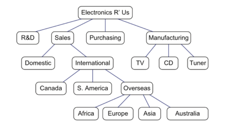
A tree is an abstract data type that stores elements hierarchically. With the exception of the top element, each element in a tree has a parent element and zero or more children elements. A tree is usually visualised by placing elements inside ovals or rectangles, and by drawing the connections between parents and children with straight lines. We typically call the top element the root of the tree, but it is drawn as the highest element, with the other elements being connected below (just the opposite of a botanical tree).

Tree Definition

A tree T is defined as a set of nodes storing elements in a parent-child relationship with the following properties:

• If T is nonempty, it has a special node, called the root of T, that has no parent.
• Each node v of T different from the root has a unique parent node w; every node with parent w is a child of w.

Note that according to our definition, a tree can be empty, meaning that it doesn’t have any nodes. This convention also allows us to define a tree recursively, such that a tree T is either empty or consists of a node r, called the root of T, and a (possibly empty) set of trees whose roots are the children of r.

Two nodes that are children of the same parent are siblings. A node v is external if v has no children. A node v is internal if it has one or more children. External nodes are also known as leaves.

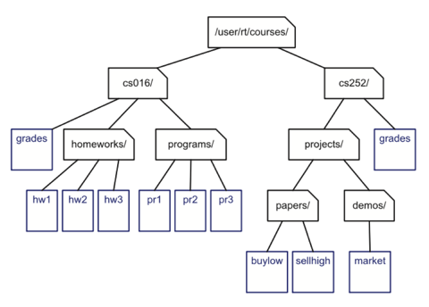
In most operating systems, files are organised hierarchically into nested directories (also called folders), which are presented to the user in the form of a tree. More specifically, the internal nodes of the tree are associated with directories and the external nodes are associated with regular files. In the UNIX and Linux operating systems, the root of the tree is appropriately called the “root directory,” and is represented by the symbol “/.”

Edges and Paths

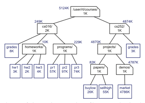
An edge of tree T is a pair of nodes (u,v) such that u is the parent of v, or vice versa. A path of T is a sequence of nodes such that any two consecutive nodes in the sequence form an edge. For example, the tree in Figure contains the path (cs252/, projects/, demos/, market).

When using single inheritance, the inheritance relation between classes in a C++ program forms a tree. The base class is the root of the tree.

Ordered Trees

A tree is ordered if there is a linear ordering defined for the children of each node; that is, we can identify children of a node as being the first, second, third, and so on. Such an ordering is determined by how the tree is to be used, and is usually indicated by drawing the tree with siblings arranged from left to right, corresponding to their linear relationship. Ordered trees typically indicate the linear order relationship existing between siblings by listing them in a sequence or iterator in the correct order.

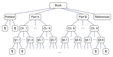
A structured document, such as a book, is hierarchically organised as a tree whose internal nodes are chapters, sections, and subsections, and whose external nodes are paragraphs, tables, figures, the bibliography, and so on. The root of the tree corresponds to the book itself. We could, in fact, consider expanding the tree further to show paragraphs consisting of sentences, sentences consisting of words, and words consisting of characters. In any case, such a tree is an example of an ordered tree, because there is a well-defined ordering among the children of each node.

Tree Traversal Algorithms

Depth and Height

Let p be a node of a tree T. The depth of p is the number of ancestors of p, excluding p itself. Note that this definition implies that the depth of the root of T is 0. The depth of p’s node can also be recursively defined as follows:

• If p is the root, then the depth of p is 0
• Otherwise, the depth of p is one plus the depth of the parent of p

Based on the above definition, the recursive algorithm depth(T, p) computes the depth of a node referenced by position p of T by calling itself recursively on the parent of p, and adding 1 to the value returned.
Algorithm depth(T, p): if p.isRoot() then return 0 else return 1 + depth(T , p.parent())The height of a tree T is the height of the root of T . In addition, height can also be viewed as the maximum depth of its external nodes.
Algorithm height1(T ): h=0 for each p ∈ T.positions() do if p.isExternal() then h = max(h, depth(T , p)) return h
This algorithm uses the depth algorithm presented earlier and is not very efficient. A more efficient algorithm is to recursively invoke the height algorithm
Algorithm height2(T, p): if p.isExternal() then return 0 elseh=0 for each q ∈ p.children() doh = max(h,height2(T,q)) return 1 + hPreorder Traversal
A traversal of a tree T is a systematic way of accessing, or “visiting,” all the nodes of T. In this section, we present a basic traversal scheme for trees, called pre- order traversal.

In a preorder traversal of a tree T, the root of T is visited first and then the subtrees rooted at its children are traversed recursively. If the tree is ordered, then the subtrees are traversed according to the order of the children. The specific action associated with the “visit” of a node depends on the application of this traversal, and could involve anything from incrementing a counter to performing some complex computation for this node. The pseudo-code for the preorder traversal of the subtree rooted at a node referenced by position p is shown below. We initially invoke this routine with the call preorder(T,T.root()).
Algorithm preorder(T, p): perform the “visit” action for node p for each child q of p do recursively traverse the subtree rooted at q by calling preorder(T,q)
The preorder traversal algorithm is useful for producing a linear ordering of the nodes of a tree where parents must always come before their children in the ordering. Such orderings have several different applications.

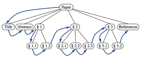
The preorder traversal of the tree associated with a document, examines an entire document sequentially, from beginning to end. If the external nodes are removed before the traversal, then the traversal examines the table of contents of the document.

Postorder Traversal

Another important tree traversal algorithm is the postorder traversal. This algorithm can be viewed as the opposite of the preorder traversal, because it recursively traverses the subtrees rooted at the children of the root first, and then visits the root. It is similar to the preorder traversal, however, in that we use it to solve a particular problem by specialising an action associated with the “visit” of a node p. Still, as with the preorder traversal, if the tree is ordered, we make recursive calls for the children of a node p according to their specified order. Pseudo-code for the postorder traversal is given below:
Algorithm postorder(T, p): for each child q of p do recursively traverse the subtree rooted at q by calling postorder(T,q) perform the “visit” action for node p

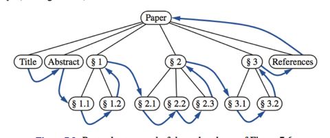
The postorder traversal method is useful for solving problems where we wish to compute some property for each node p in a tree, but computing that property for p requires that we have already computed that same property for p’s children. Such an application is illustrated in the following example.
Consider a file-system tree T, where external nodes represent files and internal nodes represent directories. Suppose we want to compute the disk space used by a directory, which is recursively given by the sum of the following:

• The size of the directory itself
• The sizes of the files in the directory
• The space used by the children directories

This computation can be done with a postorder traversal of tree T. After the subtrees of an internal node p have been traversed, we compute the space used by p by adding the sizes of the directory p itself and of the files contained in p, to the space used by each internal child of p, which was computed by the recursive postorder traversals of the children of p.

Other Kinds of Traversals

Preorder traversal is useful when we want to perform an action for a node and then recursively perform that action for its children, and postorder traversal is useful when we want to first perform an action on the descendants of a node and then perform that action on the node.

Although the preorder and postorder traversals are common ways of visiting the nodes of a tree, we can also imagine other traversals. For example, we could traverse a tree so that we visit all the nodes at depth d before we visit the nodes at depth d + 1. Such a traversal, called a breadth-first traversal, could be implemented using a queue, whereas the preorder and postorder traversals use a stack. (This stack is implicit in our use of recursion to describe these functions, but we could make this use explicit, as well, to avoid recursion.) In addition, binary trees, support an additional traversal method known as the inorder traversal.

Binary Trees

A binary tree is an ordered tree in which every node has at most two children.

1. Every node has at most two children.
2. Each child node is labeled as being either a left child or a right child.
3. A left child precedes a right child in the ordering of children of a node.

The subtree rooted at a left or right child of an internal node is called the node’s left subtree or right subtree, respectively. A binary tree is proper if each node has either zero or two children. Some people also refer to such trees as being full binary trees. Thus, in a proper binary tree, every internal node has exactly two children. A binary tree that is not proper is improper.

An important class of binary trees arises in contexts where we wish to represent a number of different outcomes that can result from answering a series of yes-or-no questions. Each internal node is associated with a question. Starting at the root, we go to the left or right child of the current node, depending on whether the answer to the question is “Yes” or “No.” With each decision, we follow an edge from a parent to a child, eventually tracing a path in the tree from the root to an external node. Such binary trees are known as decision trees, because each external node p in such a tree represents a decision of what to do if the questions associated with p’s ancestors are answered in a way that leads to p. A decision tree is a proper binary tree. Figure illustrates a decision tree that provides recommendations to a prospective investor.


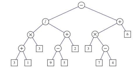
An arithmetic expression can be represented by a tree whose external nodes are associated with variables or constants, and whose internal nodes are associated with one of the operators +, −, ×, and /. Each node in such a tree has a value associated with it.

• If a node is external, then its value is that of its variable or constant.
• If a node is internal, then its value is defined by applying its operation to the values of its children.

Such an arithmetic-expression tree is a proper binary tree, since each of the operators +, −, ×, and / take exactly two operands. Of course, if we were to allow for unary operators, like negation (−), as in “−x,” then we could have an improper binary tree.

A Recursive Binary Tree Definition

Incidentally, we can also define a binary tree in a recursive way such that a binary tree is either empty or consists of:

• A node r, called the root of T and storing an element
• A binary tree, called the left subtree of T
• A binary tree, called the right subtree of T

Properties of Binary Trees

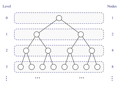
Binary trees have several interesting properties dealing with relationships between their heights and number of nodes. We denote the set of all nodes of a tree T , at the same depth d, as the level d of T. In a binary tree, level 0 has one node (the root), level 1 has, at most, two nodes (the children of the root), level 2 has, at most, four nodes, and so on. In general, level d has, at most, 2^d nodes.

A Linked Structure for Binary Trees

A binary tree T can be implemented as a linked structure. We represent each node v of T by a node object storing the associated element and pointers to its parent and two children. For simplicity, we assume the tree is proper, meaning that each node has either zero or two children.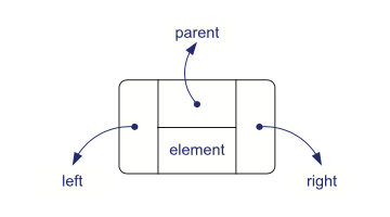

Figure below shows a linked structure representation of a binary tree. The structure stores the tree’s size, that is, the number of nodes in the tree, and a pointer to the root of the tree. The rest of the structure consists of the nodes linked together appropriately. If v is the root of T, then the pointer to the parent node is nullptr, and if v is an external node, then the pointers to the children of v are nullptr.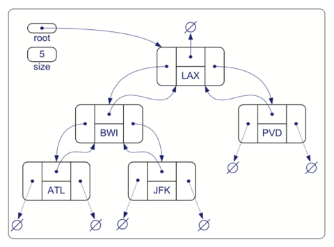

Traversals of a Binary Tree

As with general trees, binary-tree computations often involve traversals.

Preorder Traversal of a Binary Tree

Since any binary tree can also be viewed as a general tree, the preorder traversal for general trees can be applied to any binary tree. We can simplify the algorithm in the case of a binary-tree traversal, however, as we show in pseudocode.
Algorithm binaryPreorder(T, p): perform the “visit” action for node p if p is an internal node then binaryPreorder(T, p.left()) {recursively traverse left subtree} binaryPreorder(T, p.right()) {recursively traverse right subtree}For example, a preorder traversal of the binary tree shown above visits the nodes in the order ⟨LAX, BWI, ATL, JFK, PVD⟩.

Postorder Traversal of a Binary Tree

Analogously, the postorder traversal for general trees (Code Fragment 7.12) can be specialized for binary trees as shown in pseudocode below.
A postorder traversal of the binary tree shown in Figure 7.14 visits the nodes in the order ⟨ATL,JFK,BWI,PVD,LAX⟩.
Algorithm binaryPostorder(T, p): if p is an internal node then binaryPostorder(T, p.left()) {recursively traverse left subtree} binaryPostorder(T, p.right()) {recursively traverse right subtree} perform the “visit” action for the node pInorder Traversal of a Binary Tree
An additional traversal method for a binary tree is the in-order traversal. In this traversal, we visit a node between the recursive traversals of its left and right sub- trees. The in-order traversal of the subtree rooted at a node p in a binary tree T is given in pseudocode.
Algorithm inorder(T, p): if p is an internal node then inorder(T, p.left()) {recursively traverse left subtree} perform the “visit” action for node p if p is an internal node then inorder(T, p.right()) {recursively traverse right subtree}For example, an in-order traversal of the binary tree shown above visits the nodes in the order ⟨ATL, BWI, JFK, LAX, PVD⟩. The in-order traversal of a binary tree T can be informally viewed as visiting the nodes of T “from left to right.” Indeed, for every node p, the in-order traversal visits p after all the nodes in the left subtree of p and before all the nodes in the right subtree of p.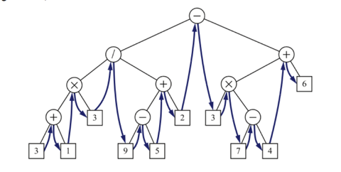


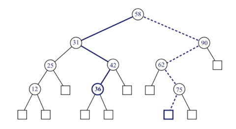
Let S be a set whose elements have an order relation. For example, S could be a set of integers. A binary search tree for S is a proper binary tree T such that:

• Each internal node p of T stores an element of S, denoted with x(p)
• For each internal node p of T , the elements stored in the left subtree of p are less than or equal to x(p) and the elements stored in the right subtree of p are greater than or equal to x(p)
• The external nodes of T do not store any element
  An in-order traversal of the internal nodes of a binary search tree T visits the elements in nondecreasing order.

We can use a binary search tree T to locate an element with a certain value x by traversing down the tree T . At each internal node we compare the value of the current node to our search element x. If the answer to the question is “smaller,” then the search continues in the left subtree. If the answer is “equal,” then the search terminates successfully. If the answer is “greater,” then the search continues in the right subtree. Finally, if we reach an external node (which is empty), then the search terminates unsuccessfully.
Note that the time for searching in a binary search tree T is proportional to the height of T. Hence, binary search trees are most efficient when they have small height.

Balanced Binary Tree

A simple binary tree without any special logic will degenerate to a linked list if data is added to the tree in sequence. Different tree implementations have been developed to solve this problem and ensure that a binary tree is balanced (ensure that finding elements in a tree has same performance characteristic of binary search).

• Randomised Binary Tree - Generate a random number and take the remainder (modulo operator) of dividing the random number by the size of the tree.
  
  
  
  • If 0 (randomly generated number is divisible by size), make the new element the root node.
  
  
  • If non-zero follow normal binary tree insertion logic to insert into either the left or right sub-tree of the root node.
    
  
  


• AVL Tree - Developed by two Soviet computer scientists, G. M. Adelson-Velskii and E. M. Landis in 1962. AVL trees are balanced in a way that for any tree node the height of its right subtree differs from the left subtree height for no more than one. Since all major operations on a BST (search, insertion and deletion) depend linearly on its height, we get a guaranteed logarithmic dependence of these algorithms operation time from the number of keys that are stored in a tree.


• Red-Black (RB) Tree - Most standard library (Java/C++) implementations use this implementation. Each node of the binary tree has an extra bit, and that bit is often interpreted as the color (red or black) of the node. These color bits are used to ensure the tree remains approximately balanced during insertions and deletions.
  
  Balance is preserved by painting each node of the tree with one of two colors (typically called 'red' and 'black') in a way that satisfies certain properties, which collectively constrain how unbalanced the tree can become in the worst case. When the tree is modified, the new tree is subsequently rearranged and repainted to restore the coloring properties. The properties are designed in such a way that this rearranging and recoloring can be performed efficiently.
  
  

Trie

A Trie, (also known as a digital/radix/prefix tree) is a special type of tree used to store associative data structures

A trie (pronounced try) gets its name from retrieval — its structure makes it a stellar matching algorithm. A trie stores data in “steps”. Each step is a node in the trie.

Storing words is a perfect use case for this kind of tree, since there are a finite amount of letters that can be put together to make a string.

Each step, or node, in a language trie will represent one letter of a word. The steps begin to branch off when the order of the letters diverge from the other words in the trie, or when a word ends.

The main idea of the trie data structure consists of the following parts:

• The trie is a tree where each vertex represents a single word or a prefix.
• The root represents an empty string (“”), the vertices that are direct children of the root represent prefixes of length 1, the vertices that are 2 edges of distance from the root represent prefixes of length 2, the vertices that are 3 edges of distance from the root represent prefixes of length 3 and so on. In other words, a vertex that are k edges of distance of the root have an associated prefix of length k.
• Let v and w be two vertexes of the trie, and assume that v is a direct parent of w, then v must have an associated prefix of w.

The next figure shows a trie with the words “tree”, “trie”, “algo”, “assoc”, “all”, and “also.”

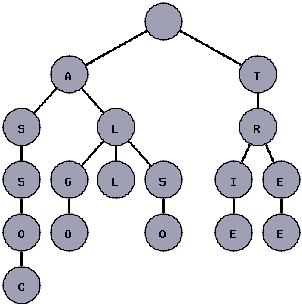
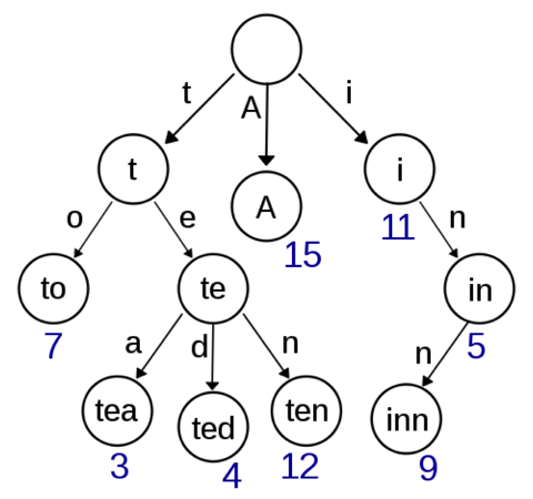
Note that every vertex of the tree does not store entire prefixes or entire words. The idea is that the program should remember the word that represents each vertex while lower in the tree.

References

http://www.sourcetricks.com/2011/06/c-tries.html
https://secweb.cs.odu.edu/~zeil/cs361/web/website/Lectures/treetraversal/page/treetraversal.html
http://www.algolist.net/Data_structures/Binary_search_tree/Removal

• You are here → 
• Home » 
• Documentation » 
• C++ Development » 
• Advanced Computer Science » 
• Lesson 17 - Tree »